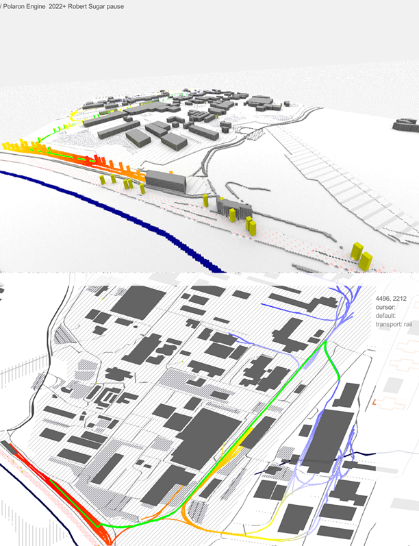
Example GeoSemantic Pipeline
1
Billions of Nodes & Points
Showing roads, Types, names and even infrastructure that we map, compare and clean and convert to Trillions of individual points – if a DEM, Lidar or equivalent map is available we will map this to 3D.
2
We convert to Trillions of Voxels
Allowing every 1m2 of a whole country to be unpacked and data added, as well as streaming in live data and running real-time queries and interactions.
3
Producing a real-time raster / simulation layer.
Blending EOS & Live Data and Cellular Automata and Agents to derive insight and calculations drive behaviours and also the foundation for synthetic terrain generation and segmentation.
4
Allowing us to simulate what is and what might be.
Based on a fusion of GIS and Live, Historic, Assumed, Observed, Pattern of life, and known vs simulated data (and we can differentiate those too).
5
Bringing real-time analysis and game experiences into real-time
With unparalleled complexity and consequence of action experiences, creating a street view based on data.
6
Which produce a giant sandbox
Providing a Sandbox of Geospatial data & allowing the Actions and Reactions of those entities and actors in the scene, giant robot fights in real life locations, planning and disaster response and more.
Open Street Map – is one of the largest semantic DB’s in the world. But we’ve used many other databases, from Ordnance Survey data to hand made KML maps and GeoJSON and more. Ultimately so long as we can interpret the data we can use and add this data into the Semantic terrain layer (ie stuff and things).
How we use Cellular Automata
There’s a brief explanation of Cellular Automata below – however in brief – we use Cellular Automata to traverse both along data types as well as to trigger relationships between entities. For instance following a route, or propagating out across all possible paths.
If for instance the route features traffic – this can be factored into the response. This allows for the Cellular Automata to be able to respond to the semantic voxels – and even interact or change them – at scale and en masse.
Each Cellular Automata isn’t in and of itself very intelligent, however a range of rules and combinations of both Cellular Automata, defined rules and other query and interaction methods lead to realistic behaviour – and indeed emergent behaviours. There is a more detailed explanation and use case below.
Cellular Automata in brief
(NB: If you’re already familiar with Cellular Automata – you can skip this)
Cellular automata are mathematical models that exhibit complex behaviours arising from simple rules. They consist of a grid of cells, each of which can be in one of a finite number of states.
https://conwaylife.com/wiki/Gosper_glider_gun
The state of each cell evolves over time based on its current state and the states of its neighbouring cells. One example of cellular automata is Conway’s Game of Life. In this cellular automaton, each cell can be either alive or dead, and the state of each cell in the next generation is determined by a set of fairly simple rules.
However through this – the interactions of different points can be calculated and when chained together with other types of Cellular Automata and related programmatic calculations – can produce emergent behaviours and effects – able to be leveraged to produce useful simulations and estimations.
Conway’s
Game of Life Rules
- Any live cell with fewer than two live neighbours dies, as if by underpopulation.
- Any live cell with two or three live neighbours lives on to the next generation.
- Any live cell with more than three live neighbours dies, as if by overpopulation.
- Any dead cell with exactly three live neighbours becomes a live cell, as if by reproduction.
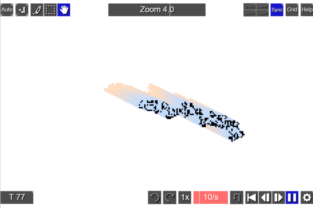
How does Polaron use Cellular Automata?
Polaron uses Cellular Automata for Propagation in both Terrain and full 3D models.
In combination with other queries and processes. The image below shows the propagation of possible paths – based on a contamination event on a Railway. This allows us to spread the “contamination” from the original source out along defined pathways.
This can be done incredibly efficiently – with a Cellular Automata being able to live profile roads and railway connections, as well as other factors (such as traffic or other interaction).
This allows us to run complex models – whereby a Cellular Automata can be used to interact with data and systems based on GIS encoded data and allows us to efficiently query and return a real-time response. From this we can then deliver data back to other systems, embedded services and even run multi-user collaborative planning applications over mobile and desktop systems – or for games to populate whole cities with infrastructure and propagate change and impacts of change along those systems.
Example of usage
Road network traversals
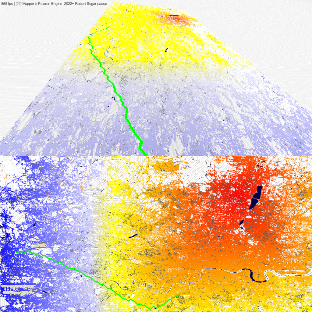
For instance, if I wanted to travel from A > B via C there are many routes I can take. We use a Dijkstra augmented Algorithm for pathing finding – but this is a small part of the process.
We can run queries from our system to quickly ingest the road status, disruptions to pathways, and add in a value (dynamic values that can change) of traffic.
We can then consider the time it takes in a cost function, with variables of the vehicle type, the cost of time and fuel to then estimate the optimal route or routes.
This approach also allows us to cache or estimate data, where there are gaps in data – or to use inference and simulation of likely conditions.
Benefits
So why is this beneficial? By comparison to other methods, this can be grown and expanded on, and bias and preference added. This allows reverse engineering of profiles of behaviour back into a Cellular Automata model – that is sufficiently representative of real-world behaviours to be a useful representation.
In effect we are using Cellular Automata as an efficient way to produce a mass agent based model. We can also introduce spawning and chaos agents – to produce random and characteristic based behaviour.
Variables
- Roads & Road Type
- Disruptions to pathways
(e.g. Road closure) - Attenuations of pathing
(e.g. Traffic) - Goals (e.g. time / fuel cost)
Cellular Interactions in 3D
Polaron’s two flavours – full volumetric and terrain models are based on the same technology applied for different types of data (we don’t for instance always need to know what is underground or flying high above us) so can exchange scales and the size of the volume instantiated and have even more processed “off map / off screen” and yet still factor into the overall simulation.
A good example of Cellular Automata is propagation & radiation.
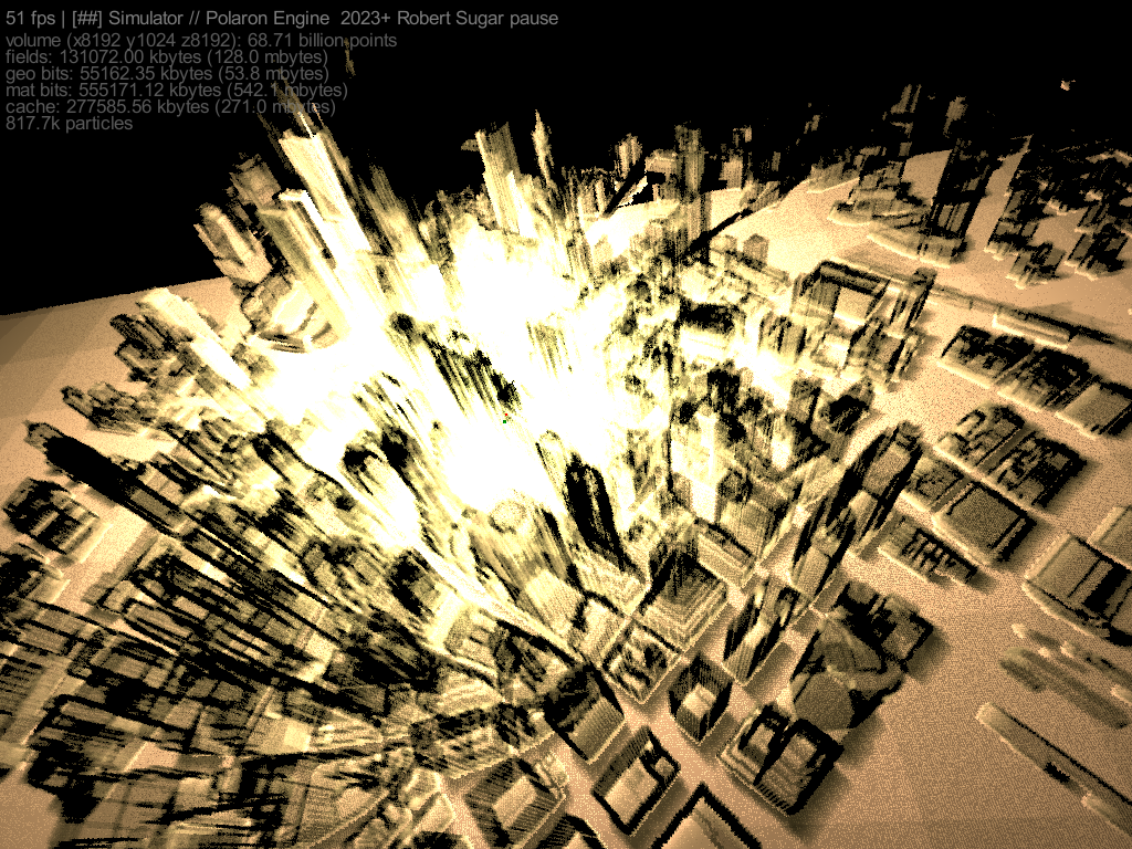
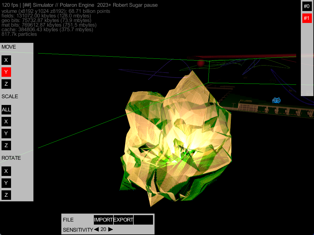
Radiation Propagation
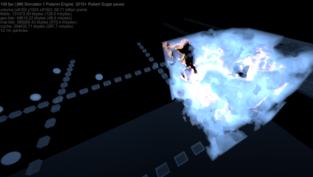
We created a block of voxels that reacts to each impact from a radiating source.
ach point in the block reacts to the impact of a radiating source that is orbiting the voxel block. As each ray hits the source it has been programmed to react and cause a decay. This produces a visual change in the output – based on a programmatic calculation of change from each impact, as well as dependencies between cells.
These can all be tuned and interacted with and secondary effects added (similar to how fire spreads or Physics interactions occur). This produces a very organic and natural interface between an emitter and an object and can be used to simulate the impact and effect of a variety of physical interactions, propagation of Radiation and RF through different materials since each cell’s effect can be processed.
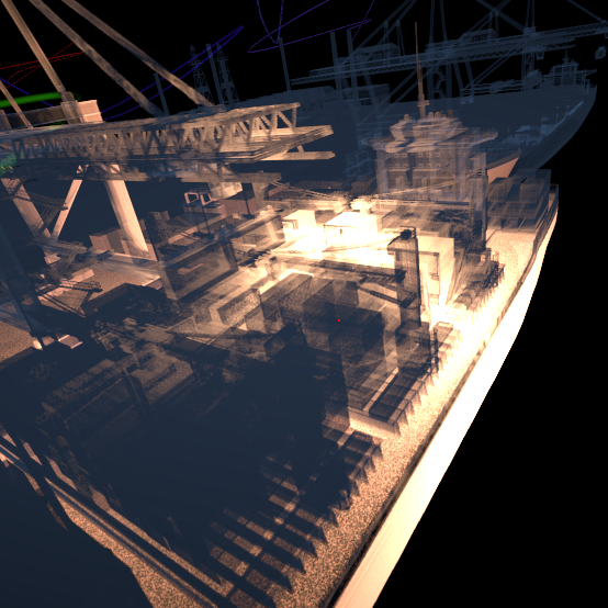
We have used Lidar scans to base this on as well – using assumed material values (reinforced concrete) as a base value for the attenuation of a given source. A tech demo of this based on a scan of the M-Shed Museum in Bristol can be seen below.
Benefits
This approach allows us to simulate emitters and can augment ray casting and marching cube approaches to allow complex interactions between emitters and material properties of different values.
Variables
- Radiating source type
- Intensity & Range
- Impact & Scattering
- Inter-cellular dependency
- Visual change
- Decay rate
- Density of object
Interactive effects
- Direction
- Force and sustainment (i.e. absorption into the material)
- Luminoscity
- Transparency & Opacity
- Interaction with neighbouring cells
- Secondary radiation (ie the first point is given a charge / emitting value)
Tests & Demos
- Light penetration and propagation into a scene
- Lidar derived penetration estimation
- Consideration of propagation into a scene and cannalising
- Representative attenuation (*ie add in transparent blocks in the volume that don’t occupy physical space visually but can warp the scene and propagation).
Propagation of effects
By using a combination of techniques it then becomes possible to represent complex events, propagation of effects, connectivity, line of sight and more. With the addition of Physics – this grows to produce highly dynamic simulations that can be used to drive real-world simulations and events.
To do this we need to then consider a range of other factors – such as the type of emission, type of propagation, and whether a Cellular Automata is the most appropriate method. We have for instance explored the use of an RF Lobe’s effect on the propagation and wave pattern through a space and whilst we’re not “RF Guys” – it seems promising as a means to shape the pattern of throw and projection into a 3D volume and the shaping of the resulting SPLAT and Connectivity patterns.
We’re currently looking at the various properties that can be encoded into the materials and terrain layer to further augment such modelling.
Variables
- Impact of change on a scene
- Effect of physics
- Intensity & Range
- Impact & Scattering
- Inter-cellular dependency
- Visual change
- Communication links
- Visibility
- Line of Sight
- Perception area
Interactive effects
- RF connection and communication
- Lines of communication
- Navigation over destroyed terrain
- Interactive elements
- System damage